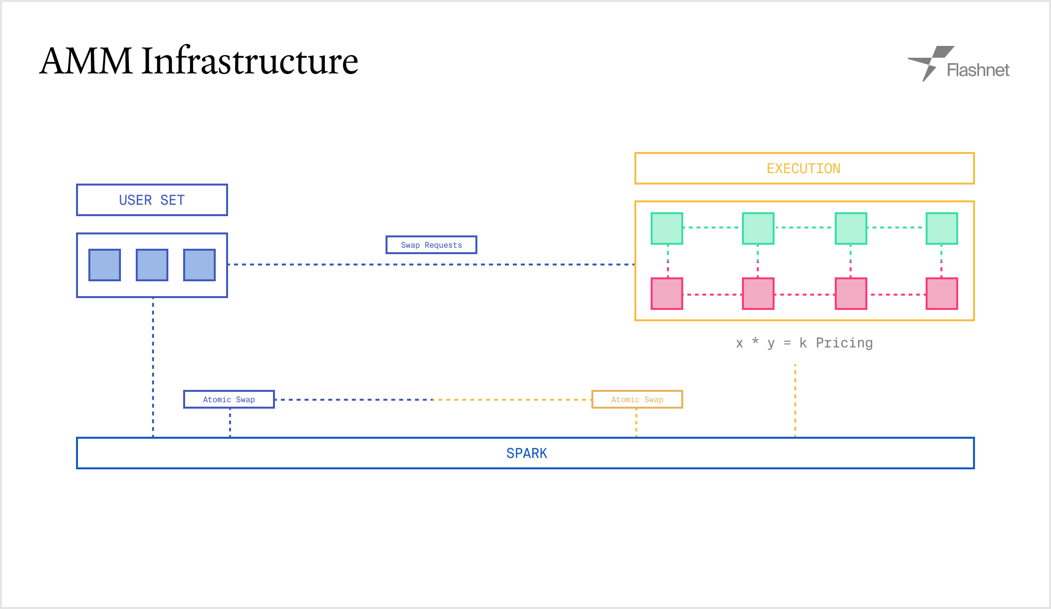
Constant Product AMM
The constant product AMM is a simpley * x = k curve that allows users to deposit two assets and enable them to be traded against each other. The price of the assets is determined by the ratio of the two assets in the pool.
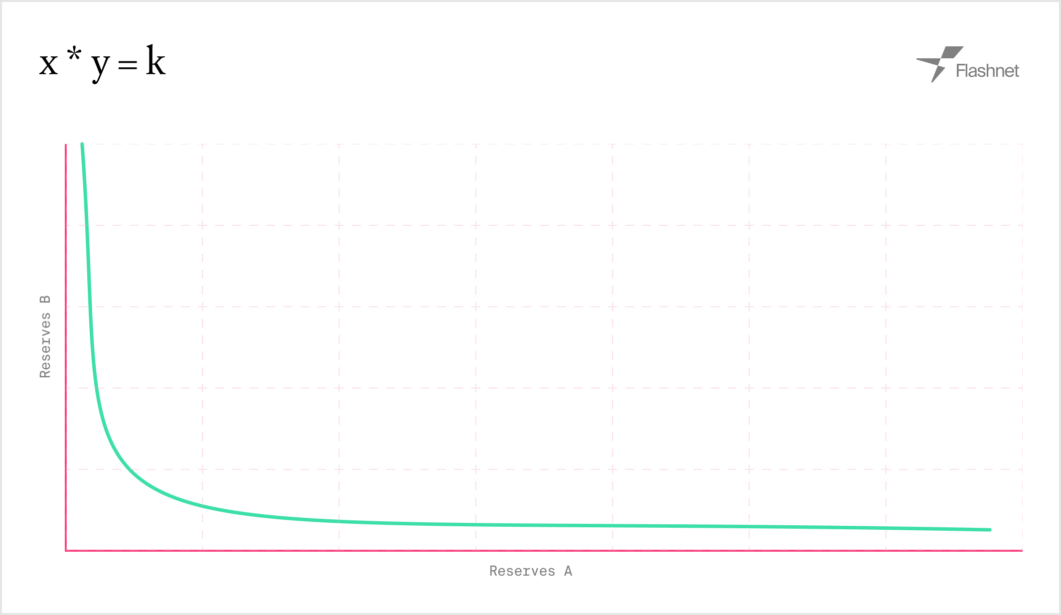
- Price(A) = Reserve_B / Reserve_A
- Trade execution follows:
(Reserve_A + ΔA - fees) * (Reserve_B - ΔB) = kwhere k is the constant product of the reserves.
Bonding Curve AMM (Single-Sided)
The single-sided AMM uses a bonding curve for gradual price discovery, making it ideal for launching new tokens. It allows a creator to supply tokens and define a price curve that evolves as the tokens are sold. Once a certain amount of the supply is sold, the pool “graduates” into a standard constant product AMM.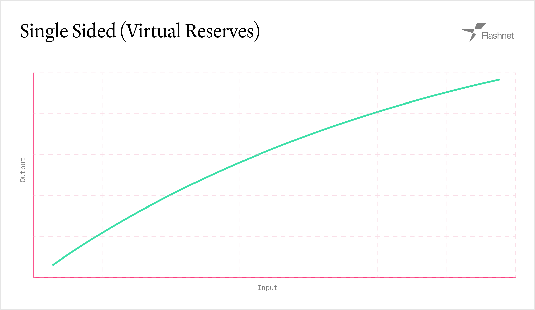
Price Mechanism
We model single‑sided sales with virtual reserves that sit on a constant‑product curve. Let initial virtual reserves bev_A^0 and v_B^0 with k_v = v_A^0 * v_B^0. As tokens are sold, we maintain:
current_v_a = v_A^0 - tokens_soldcurrent_v_b = v_B^0 + quote_raised
P = current_v_b / current_v_a
Swaps update virtual reserves using constant product math:
- Buy A with B (B→A):
new_v_b = current_v_b + ΔB,new_v_a = k_v / new_v_b, outputΔA = current_v_a - new_v_a. - Sell A for B (A→B):
new_v_a = current_v_a + ΔA,new_v_b = k_v / new_v_a, outputΔB = current_v_b - new_v_b.
Concentrated Liquidity AMM
The concentrated liquidity AMM implementation allows liquidity providers to concentrate their capital within specific price ranges, similar to Uniswap V3. This enables more capital-efficient liquidity provision compared to traditional constant product AMMs.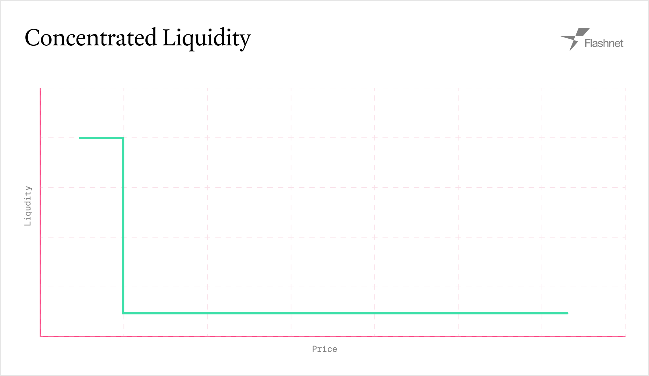
-
Liquidity Calculation:
- Below range:
L = (ΔA * sqrt(P_upper) * sqrt(P_lower)) / (sqrt(P_upper) - sqrt(P_lower)) - Above range:
L = ΔB / (sqrt(P_upper) - sqrt(P_lower)) - Within range:
L = min(L_A, L_B)where both assets may be required
- Below range:
- Swap Execution: Swaps traverse tick boundaries, activating/deactivating liquidity as price moves
- Fee Growth Tracking: Global and per-position fee growth is tracked for accurate fee distribution